The Autonomy Governor: Risk Score Construction, Calibration, and Failure Modes

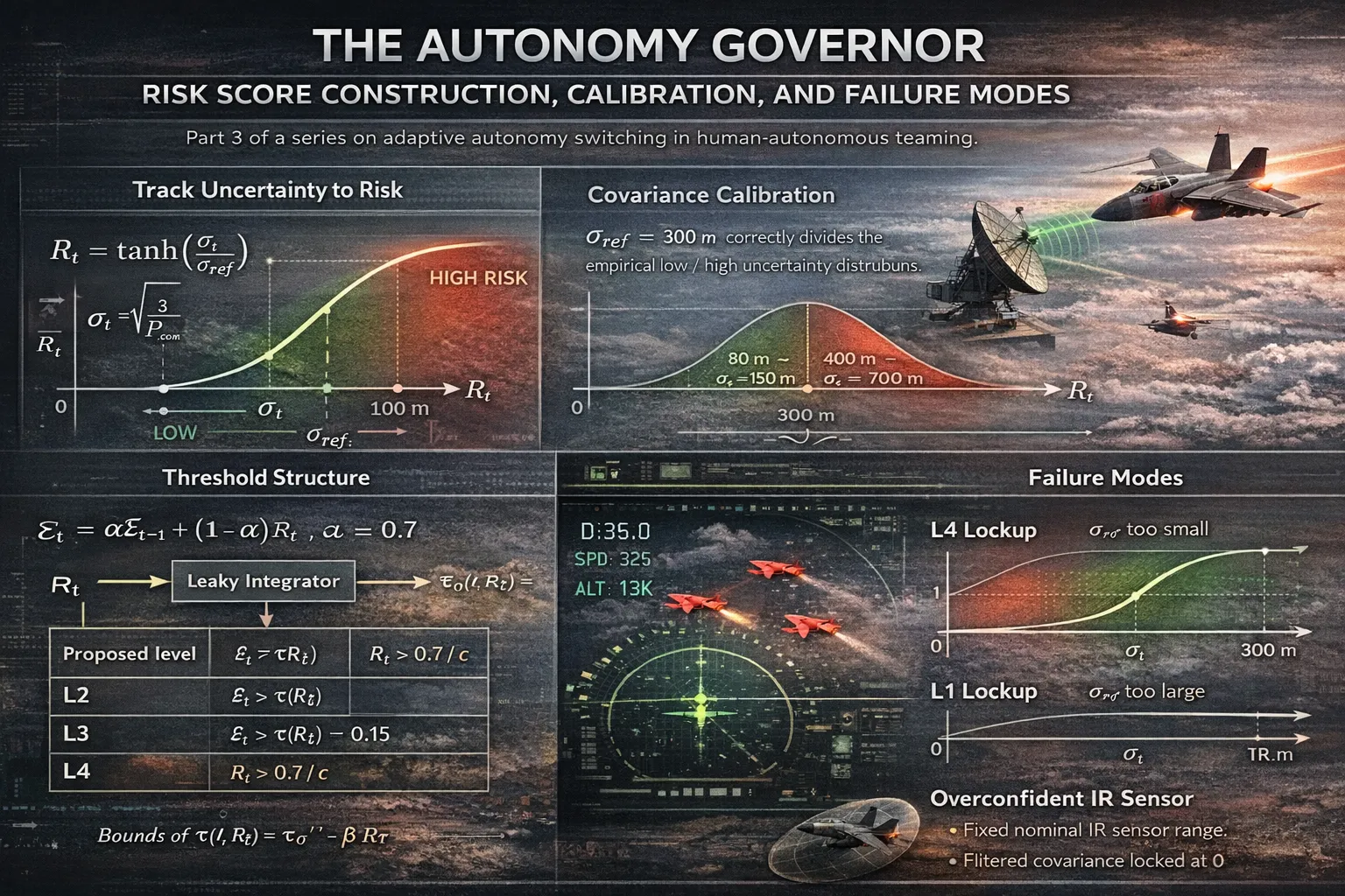
Part 3 of a series on adaptive autonomy switching in human-autonomous teaming.

---

From Track Uncertainty to Risk

The fusion pipeline produces, at each timestep $t$, a fused position covariance $\mathbf{P}_t^{\mathrm{pos}} \in \mathbb{R}^{3\times3}$. The governor’s first task is to distill this into a scalar risk signal $R_t \in [0,1]$. The chosen mapping is:

$R_t = \tanh\!\left(\frac{\sigma_t}{\sigma_{\mathrm{ref}}}\right), \quad \sigma_t = \sqrt{\frac{1}{3}\, \operatorname{tr}(\mathbf{P}_t^{\mathrm{pos}})}$

The $\tanh$ is not arbitrary. It has three properties that matter here:

1. Bounded output: $R_t \in (0,1)$ regardless of how large $\sigma_t$ gets, so a diverging tracker does not produce unbounded risk estimates.
2. Monotone sensitivity: $\partial R_t / \partial \sigma_t > 0$ everywhere, so improvements in tracking quality are always reflected in the risk signal.
3. Saturation at both ends: for $\sigma_t \ll \sigma_{\mathrm{ref}}$, $R_t \approx \sigma_t / \sigma_{\mathrm{ref}}$ (linear, sensitive); for $\sigma_t \gg \sigma_{\mathrm{ref}}$, $R_t \to 1$ (saturated, stable). This means the governor does not continue differentiating between “bad” and “catastrophic” tracker states once the track has effectively failed, the risk is maximal and the response is the same.

The calibration constant $\sigma_{\mathrm{ref}}$ sets the inflection point of the $\tanh$ the uncertainty value at which the governor is operating in its most sensitive regime. Choosing it correctly is the central calibration problem.

---

The Calibration Problem

The initial value of $\sigma_{\mathrm{ref}}$ was set to 50 m, chosen intuitively as “roughly the radar range noise.” This was wrong, and the consequences were total.

With $\sigma_{\mathrm{ref}} = 50$ m, a tracker with $\sigma_t = 100$ m produces $R_t = \tanh(2) \approx 0.96$ near-maximum risk at all times, regardless of scenario conditions. The governor locked at $L_4$ for every policy and every sensor quality condition. The experimental design had $\Delta\ell \approx 0$ across all policies, indistinguishable from a fixed-$L_4$ policy. There was no signal to find.

The correct approach is to calibrate $\sigma_{\mathrm{ref}}$ against the actual distribution of $\sigma_t$ values produced by the pipeline. Running the sensor stack under nominal (HIGH quality) conditions produces a convergent tracker with $\sigma_t \in [80, 150]$ m. Under degraded (LOW quality) conditions, $\sigma_t$ ranges over $[400, 700]$ m with intermittent dropouts. The $\tanh$ inflection should sit somewhere in the middle of this range not below the minimum, not above the maximum.

Setting $\sigma_{\mathrm{ref}} = 300$ m places the inflection point at the boundary between HIGH and LOW quality regimes:

$R_t\big(\sigma_t = 100\,\mathrm{m}\big) = \tanh(0.33) \approx 0.32 \quad (\text{LOW risk - HIGH quality sensor})$

$R_t\big(\sigma_t = 500\,\mathrm{m}\big) = \tanh(1.67) \approx 0.93 \quad (\text{HIGH risk - LOW quality sensor})$

This spread is what the experiment needs. At $\sigma_{\mathrm{ref}} = 50$ m, both values map to $R_t \approx 1$; at $\sigma_{\mathrm{ref}} = 300$ m, they map to $\{0.32, 0.93\}$ - a range that drives meaningful threshold variation through $\tau(\ell, R_t) = \tau_0^\ell - \beta R_t$.

The general principle: $\sigma_{\mathrm{ref}}$ must be calibrated against the empirical covariance distribution of your specific tracker and sensor configuration, not derived from sensor noise parameters alone. The relationship between measurement noise, process noise, filter gain, and steady-state covariance is nonlinear and cannot be reliably estimated without running the filter.

---

Evidence Accumulation

Rather than applying $R_t$ to the threshold directly, the governor accumulates a leaky-integrated evidence signal:

$\mathcal{E}_t = \alpha\, \mathcal{E}_{t-1} + (1-\alpha)\, R_t, \quad \alpha = 0.7$ $\mathcal{E}_t = \alpha\, \mathcal{E}_{t-1} + (1-\alpha)\, R_t, \quad \alpha = 0.7$

This is a first-order IIR filter on the risk signal. The time constant is $\tau_e = -\Delta t / \ln(\alpha) \approx 3$ steps at $\Delta t = 0.05$ s about 150 ms. This serves two purposes. First, it suppresses transient spikes in $R_t$ caused by individual missed detections or single-step covariance blowups. Second, it enforces an implicit dwell time: the evidence cannot change faster than the filter’s time constant, which bounds the switching rate.

Note the difference from the sliding-window formulation in Part 1. A sliding window of length $W$ gives equal weight to all $W$ past observations and zero weight to older ones a rectangular impulse response. The leaky integrator gives exponentially decaying weight to past observations with no sharp cutoff. In practice the leaky integrator is more numerically stable and easier to tune with a single parameter ($\alpha$).

---

The Threshold Structure

With $\mathcal{E}_t$ and $R_t$ in hand, the level selection follows:

tau = TAU0 if policy == 'evidence_only' else TAU0 - BETA * R_t

if evidence > tau:           proposed = 2
if evidence > tau - 0.15:    proposed = 3
if R_t > 0.7 / crit_mult:    proposed = 4

with TAU0 = 0.6, BETA = 0.3. The level-specific thresholds are:

Proposed level	Condition
L2	$\mathcal{E}_t > \tau(R_t)$
L3	$\mathcal{E}_t > \tau(R_t) - 0.15$
L4	$R_t > 0.7 / c$

where $c$ is the mission criticality multiplier. The L4 condition is driven directly by $R_t$ rather than $\mathcal{E}_t$ when risk is sufficiently high, accumulated evidence is irrelevant. The mission criticality parameter shifts this threshold: $c = 1.5$ (HIGH criticality) lowers the L4 threshold to $0.47$, escalating to full autonomy earlier; $c = 0.5$ (LOW criticality) raises it to $1.4$, which is above the maximum value of $R_t \in (0,1)$ and effectively disables L4 escalation in low-stakes scenarios.

This last point was the source of a sign-inversion bug. The original implementation used R_t > 0.7 * crit_mult instead of R_t > 0.7 / crit_mult. With the multiplication form, HIGH criticality raised the threshold (harder to reach L4), and LOW criticality lowered it exactly backwards. The direction of the effect was correct in the evidence terms but inverted in the risk-override term. The bug was invisible in aggregate metrics (because $\Delta\ell$ is computed over all criticality conditions) and only surfaced when stratifying results by mission criticality, where the sign of the adaptation effect was reversed.

---

Hysteresis

A bare threshold produces chattering rapid oscillation between adjacent levels when $\mathcal{E}_t$ hovers near $\tau$. The standard fix is hysteresis: downward transitions are blocked unless the governor has spent at least HYSTERESIS = 5 steps at the current level.

if proposed > prev_level:
    new = proposed                          # upward: immediate
elif proposed < prev_level:
    new = proposed if steps_at_level >= HYSTERESIS else prev_level
else:
    new = prev_level

Upward transitions are immediate; the system escalates authority as fast as the evidence warrants. Downward transitions are delayed. This asymmetry reflects the asymmetric cost structure: failing to escalate when the situation deteriorates is more dangerous than maintaining a higher autonomy level for a few extra steps.

With HYSTERESIS = 5 at $\Delta t = 0.05$ s, the minimum dwell time before a downward transition is 250 ms. In practice the effective dwell is longer because the evidence signal must also decay through the IIR filter before proposed < prev_level becomes true.

---

The XAI Log

Every autonomy switch event is serialized to a JSONL file:

{
  "t": 47.3, "phase": "Phase2", "level": 3, "level_name": "Conditional",
  "switched": true,
  "fast_level": 3, "fast_conf": 0.82, "fast_rationale": "2 threats at 35km, R=0.71",
  "slow_level": 3, "slow_conf": 0.79,
  "slow_summary": "Two converging hostiles at medium range with degraded track quality.",
  "slow_visual": "Tracks converging in upper-left quadrant.",
  "R": 0.712, "sigma_pos_m": 387.4, "n_threats": 2
}

Non-switch steps are not logged. This keeps the log compact while preserving full fidelity on the events that matter. The log is the primary artifact for XAI analysis: for each switch, we have the reason (fast rationale + slow summary), the quantitative state that triggered it ($R_t$, $\sigma_t$, $n_{\mathrm{threats}}$), and the disagreement structure between the two deciders (fast vs. slow level).

---

What Breaks and Why

Three failure modes dominated the debugging phase.

Governor lockup at $L_4$. Caused by $\sigma_{\mathrm{ref}}$ too small. The fix is empirical calibration against the actual covariance distribution, as described above.

Governor lockup at $L_1$. The opposite failure: $\sigma_{\mathrm{ref}}$ too large (e.g., 5000 m) maps all realistic $\sigma_t$ values to $R_t \approx 0$, keeping $\tau \approx \tau_0 = 0.6$ and the evidence signal too low to cross it. The governor sees everything as low-risk and stays at the lowest level.

IR overconfidence locking the covariance. When the IR sensor model assigned a fixed nominal range to all angle-only detections, the implied position error was $\sigma_{\mathrm{pos}}^{\mathrm{IR}} \approx r_{\mathrm{nominal}} \cdot \sigma_\varphi$. At close range, this produced $\sigma_{\mathrm{pos}} < 1$ m, which propagated through the CI fusion to give $\mathbf{P}_t^{\mathrm{pos}} \approx 0$, $\sigma_t \approx 0$, $R_t \approx 0$, and permanent $L_1$. The fix enforcing $\sigma_{\mathrm{pos}}^{\mathrm{IR}}(r) = r \cdot \sigma_\varphi$ with a hard floor at sigma_pos_min = 30 m ensures the effective position uncertainty is always physically interpretable as a function of range and angular noise, and never collapses to zero regardless of sensor geometry.

All three failures produce identical observable behavior: the mean autonomy level is constant across all scenario cells, $\Delta\ell \approx 0$, and no policy differs from any other in the outcome metrics. Without knowing what the governor should be doing, these failures are silent.

---

Next: Part 4 - Monte Carlo results: the $\Delta\ell$ comparison across policies, Mann-Whitney U tests, and why the mission success metric is the wrong thing to look at.