Building the Simulation Environment: Flight Dynamics, Sensor Models, and IMM-EKF Fusion

Part 2 of a series on adaptive autonomy switching in human-autonomous teaming.

---

Why Simulation Fidelity Matters Here

The autonomy governor makes switching decisions based on a single derived quantity: track quality $q_t$, computed from the position uncertainty $\mathbf{P}_t$ of a fused state estimate. Everything upstream of the governor flight dynamics, sensor models, tracking filters, fusion exists to produce a realistic $(\mathbf{x}_t, \mathbf{P}_t)$ pair whose covariance structure reflects genuine epistemic uncertainty rather than a hand-tuned scalar.

This is a non-trivial requirement. A governor calibrated against an overly optimistic covariance will appear adaptive when it is actually operating in a permanently high-confidence regime; one calibrated against an inflated covariance will be pathologically conservative. The simulation must therefore be physically grounded enough that $\mathbf{P}_t$ responds meaningfully to the environmental factors we want to stress-test: sensor quality, threat tempo, and engagement geometry.

---

3-DOF Point Mass Dynamics

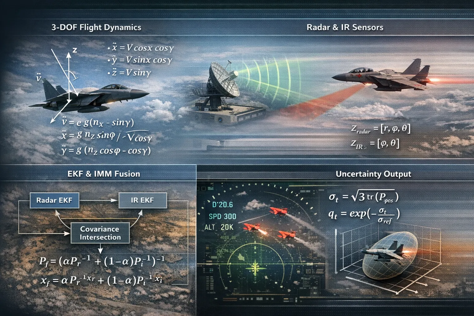
The flight environment is built on a 3-DOF point mass model, derived from a MATLAB simulation package and ported to Python. The state vector is:

$\mathbf{s} = [x,\ y,\ z,\ V,\ \chi,\ \gamma]^\top$

where $(x, y, z)$ is position in a local NED frame, $V$ is total airspeed, $\chi$ is heading angle, and $\gamma$ is flight path angle. The equations of motion follow directly from Newton’s second law applied to a point mass in coordinated flight:

$\dot{x} = V \cos\chi \cos\gamma, \quad \dot{y} = V \sin\chi \cos\gamma, \quad \dot{z} = V \sin\gamma$

$\dot{V} = g(n_X - \sin\gamma)$

$\dot{\chi} = \frac{g\, n_Z \sin\phi}{V \cos\gamma}, \quad \dot{\gamma} = \frac{g}{V}(n_Z \cos\phi - \cos\gamma)$

The control inputs are the axial load factor $n_X$, the normal load factor $n_Z$, and the bank angle $\phi$. These are driven by an autopilot layer: separate PID controllers for speed, altitude, and heading track commanded references and produce $(n_X, n_Z, \phi)$ at each timestep $\Delta t = 0.05$ s.

Different platform archetypes are modeled and each parameterized by performance envelopes: $V \in [V_{\min}, V_{\max}]$, $n_Z \in [n_{Z,\min}, n_{Z,\max}]$, and maximum bank and path angles. The fighter jet, used as the RED threat in most scenarios, has $n_{Z,\max} = 9\,g$ and $V_{\max} = 700$ m/s; its autopilot can execute sustained high-$g$ turns. This envelope determines the upper bound on threat maneuverability the tracker must accommodate.

The atmosphere model follows ISA troposphere: density and speed of sound are computed as functions of altitude up to the tropopause, providing altitude-dependent aerodynamic limits for each platform type.

---

Sensor Models

Two sensor modalities are implemented: a tracking radar and a passive IR sensor. Both operate in spherical coordinates relative to the ownship position.

Radar. The radar produces range-azimuth-elevation measurements:

$\mathbf{z}_t^{\mathrm{radar}} = \begin{bmatrix} r \\\\ \varphi \\\\ \theta \end{bmatrix} + \boldsymbol{\nu}_t, \qquad \boldsymbol{\nu}_t \sim \mathcal{N}(\mathbf{0},\, \mathbf{R}_{\mathrm{radar}})$

$\mathbf{R}_{\mathrm{radar}} = \operatorname{diag}\!\left(\sigma_r^2,\, \sigma_\varphi^2,\, \sigma_\theta^2\right)$

with $\sigma_r = 50$ m, $\sigma_\varphi = \sigma_\theta = 0.5°$ under nominal (HIGH quality) conditions; degraded (LOW quality) scenarios multiply these by a factor of 4. Detections are gated at a maximum range of 100 km. The radar is a range-complete sensor: it provides direct range information, which means its measurements can be linearized to Cartesian with bounded position error.

IR sensor. The IR sensor is angle-only:

$\mathbf{z}_t^{\mathrm{IR}} = \begin{bmatrix} \varphi \\\\ \theta \end{bmatrix} + \boldsymbol{\nu}_t, \qquad \boldsymbol{\nu}_t \sim \mathcal{N}(\mathbf{0},\, \mathbf{R}_{\mathrm{IR}})$

$\mathbf{R}_{\mathrm{IR}} = \operatorname{diag}\!\left(\sigma_\varphi^2,\, \sigma_\theta^2\right), \qquad \sigma_\varphi = \sigma_\theta = 0.2^\circ$

The absence of range information creates a fundamental observability constraint: an angle-only sensor cannot initialize a Cartesian track without auxiliary range information. In the pipeline, IR detections are used to update existing radar-initialized tracks; an IR-only detection does not open a new track. This is enforced by the track management logic described below.

A critical implementation issue emerged here. A naive IR model that assigns a nominal fixed range to each detection produces $\sigma_{\mathrm{pos}} \to 0$ at close range a geometrically impossible result that drives $q_t \to 1$ and locks the governor at $L_4$ regardless of actual tracking quality. The fix is an angular noise floor that maps angular uncertainty to a range-dependent position uncertainty:

$\sigma_{\mathrm{pos}}^{\mathrm{IR}}(r) = r \cdot \sigma_\varphi$

ensuring that the effective position uncertainty grows with range, as it physically should. This single correction was essential to prevent governor lockup.

---

EKF Tracking

Each sensor modality runs an independent EKF tracker. The state model is constant velocity (CV) in Cartesian coordinates:

$\mathbf{x}_t = \mathbf{F}(\Delta t)\,\mathbf{x}_{t-1} + \mathbf{w}_t, \quad \mathbf{w}_t \sim \mathcal{N}(\mathbf{0},\, \mathbf{Q}(\Delta t))$

$\mathbf{F}(\Delta t) = \begin{bmatrix} \mathbf{I}_3 & \Delta t\,\mathbf{I}_3 \\\\ \mathbf{0}_3 & \mathbf{I}_3 \end{bmatrix}$

The process noise $\mathbf{Q}$ follows the discrete Wiener acceleration model:

$\mathbf{Q}(\Delta t) = q \cdot \mathbf{G}\mathbf{G}^\top, \quad \mathbf{G} = \begin{bmatrix} \frac{1}{2}\Delta t^2 \\\\ \Delta t \end{bmatrix} \otimes \mathbf{I}_3$

where $q$ is the acceleration spectral density, tuned to match the maneuvering bandwidth of the RED platform.

The measurement update linearizes the spherical-to-Cartesian conversion at the predicted position. For radar, the Jacobian $\mathbf{H}$ maps the full $(r, \varphi, \theta)$ measurement to Cartesian increments; for IR angle-only updates, $\mathbf{H}$ is computed with range held fixed at the predicted track range, and the update is applied only to the angular degrees of freedom.

Track management follows a standard M-of-N confirmation / deletion logic: a new tentative track is confirmed after 3 consecutive hits, and an existing track is deleted after 10 consecutive misses. This introduces a track latency that directly affects the governor: the system cannot act on a new threat until the tracker has confirmed it, which takes $3\,\Delta t$ at minimum. At $\Delta t = 0.05$ s this is 150 ms fast enough for the engagement timescales considered here, but a genuine design constraint.

The IMM (Interacting Multiple Model) extension maintains a bank of models constant velocity and constant turn with mode probabilities updated at each step via the mixing weights:

$\mu_i^k = \frac{p_{ij}\, \mu_j^{k-1}}{\sum_j p_{ij}\, \mu_j^{k-1}}$

The mixed state and covariance are computed as weighted sums over models, providing a smoother covariance estimate during maneuvering phases than a single CV filter.

---

Covariance Intersection Fusion

The radar and IR trackers produce independent track estimates $(\mathbf{x}^r, \mathbf{P}^r)$ and $(\mathbf{x}^i, \mathbf{P}^i)$ for each platform. These are fused using Covariance Intersection (CI), which is consistent the fused covariance $\mathbf{P}^f$ is guaranteed to be an upper bound on the true covariance without requiring knowledge of the cross-correlations between the two trackers:

$\mathbf{P}^f = \left(\alpha\,(\mathbf{P}^r)^{-1} + (1-\alpha)\,(\mathbf{P}^i)^{-1}\right)^{-1}$

$\mathbf{x}^f = \mathbf{P}^f \left(\alpha\,(\mathbf{P}^r)^{-1}\mathbf{x}^r + (1-\alpha)\,(\mathbf{P}^i)^{-1}\mathbf{x}^i\right)$

The mixing weight $\alpha \in (0,1)$ minimizes $\operatorname{tr}(\mathbf{P}^f)$; in the current implementation it is fixed at $\alpha = 0.5$ as a computationally cheap approximation. The optimal $\alpha^*$ can be found by line search; given the already conservative nature of CI, the approximation error is small relative to the process noise term.

When only one sensor has a confirmed track on a given platform, the single-sensor estimate passes through without fusion. When neither sensor has a track, there is no FusedTrack for that platform, and the governor receives no evidence which correctly forces $\mathcal{E}_t$ toward zero and triggers a downward level transition.

---

The TrackOutput Interface

The output of the fusion stage is a FusedTrack dataclass:

@dataclass
class FusedTrack:
    id:          int
    t:           float
    x:           np.ndarray   # (6,): [x, y, z, vx, vy, vz]
    P:           np.ndarray   # (6, 6)
    platform_id: int

This is the only object the governor sees. The autonomy layer has no access to raw detections, individual sensor states, or platform truth a deliberate interface boundary that enforces the separation between estimation and decision. The governor operates on $(\mathbf{x}_t, \mathbf{P}_t)$ alone, extracting track quality via:

$q_t = \exp\!\left(-\frac{\sigma_t}{\sigma_{\mathrm{ref}}}\right), \quad \sigma_t = \sqrt{\frac{1}{3}\,\operatorname{tr}(\mathbf{P}_t^{\mathrm{pos}})}$

The calibration of $\sigma_{\mathrm{ref}}$ is the subject of the next post it turns out to be the single most consequential parameter in the entire system, and getting it wrong in either direction produces a governor that is observationally indistinguishable from a fixed policy.

---

What This Stack Produces

In a nominal HIGH-quality sensor scenario with a single RED threat at 40 km and closing at 300 m/s, the fused tracker converges to $\sigma_t \approx 80$–$150$ m within 5 seconds of first detection. In a LOW-quality scenario (4× noise scaling on both sensors), the same engagement produces $\sigma_t \approx 400$–$700$ m, with intermittent track drops when the IR sensor misses due to extended range gating. This spread is large enough to drive meaningful variation in $q_t$ and therefore in $\mathcal{E}_t$ across the HIGH/LOW sensor conditions, which is precisely what the experimental design requires.

The multi-threat scenarios (3 simultaneous RED platforms) produce track cross-contamination during close passes when the assignment gating radius is exceeded. This is not a bug; it is a realistic failure mode that stresses the governor in a way that is difficult to reproduce analytically.

---

Next: Part 3 - The Governor: risk score construction, $\sigma_{\mathrm{ref}}$ calibration, and the failure modes that took the longest to diagnose.