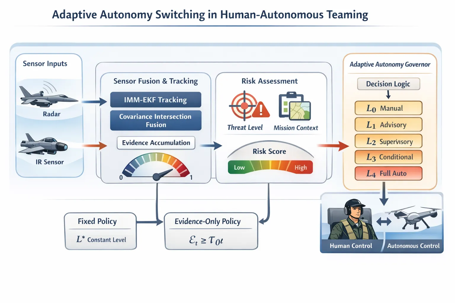
Adaptive Autonomy Switching in Human-Autonomous Teaming: Motivation and Formulation

Part 1 of a series on building and evaluating a risk-dependent autonomy governor for military aviation.

---

Problem Statement

Human-autonomous teaming (HAT) in tactical aviation faces a fundamental allocation problem: which cognitive and executive functions belong to the human, which to the machine, and crucially how should that allocation change as the operational environment evolves?

Existing approaches treat this as a threshold problem over a fixed scalar metric: track quality drops below $\epsilon$, autonomy level drops. This is brittle in two ways. First, it conflates sensor degradation with sensor failure a noisy but unbiased radar and a jammed radar demand different responses. Second, and more fundamentally, it ignores situational risk: the cost of under-automation in a terminal threat engagement is not the same as the cost in a low-threat transit leg. A threshold calibrated for one context will be miscalibrated for the other.

The question this project addresses is: can we construct an autonomy governor whose switching policy is provably adaptive to both sensor quality and tactical risk, and what is the performance gain over fixed or risk-agnostic alternatives?

---

Autonomy Levels and Transition Semantics`

We adopt a five-level taxonomy $\mathcal{L} = \{L_0, L_1, L_2, L_3, L_4\}$ aligned with the DoD autonomy framework:

Level	Designation	Human–machine authority split
$L_0$	Manual	Human executes; system observes
$L_1$	Advisory	System recommends; human decides
$L_2$	Supervisory	System acts; human monitors and overrides
$L_3$	Conditional	System acts within pre-authorized envelopes
$L_4$	Full	System acts without human input

The semantics of a transition $L_i \to L_j$ are asymmetric. Upward transitions ($j > i$) increase automation and reduce human cognitive load but increase the risk of acting on a bad estimate. Downward transitions ($j < i$) restore human authority but impose reaction-time costs that may be prohibitive at high threat tempo. A well-designed governor must minimize unnecessary transitions while remaining responsive to genuine state changes a stability-responsiveness trade-off not addressed by instantaneous thresholding.`

Evidence Accumulation

Let $\mathbf{x}_t \in \mathbb{R}^6$ be the fused track state (position + velocity) at time $t$, with associated covariance $\mathbf{P}_t \in \mathbb{R}^{6\times6}$ produced by an IMM-EKF fusion stage (described in Part 2). Define the instantaneous track quality:

$q_t = \exp!\left(-\frac{\sigma_t}{\sigma_{\mathrm{ref}}}\right), \quad \sigma_t = \sqrt{\tfrac{1}{3},\mathrm{tr}(\mathbf{P}_t^{\mathrm{pos}})}$

where $\mathbf{P}_t^{\mathrm{pos}}$ is the $3\times3$ position subblock of $\mathbf{P}_t$ and $\sigma_{\mathrm{ref}}$ is a calibration constant. This maps position uncertainty to $q_t \in (0,1]$, with $q_t \to 1$ as the tracker converges and $q_t \to 0$ as it diverges.

Rather than thresholding $q_t$ directly, the governor accumulates evidence over a sliding window of length $W$:

$\mathcal{E}_t = \frac{1}{W} \sum_{k=t-W+1}^{t} q_k$

This suppresses transient measurement outliers and introduces a lower bound on transition dwell time the governor cannot oscillate between levels faster than $W$ steps, a necessary stability condition in noisy environments.

---

Risk-Dependent Threshold

Let $R_t \in [0,1]$ be a composite risk score derived from threat proximity, closure rate, and mission phase (the precise construction of $R_t$ is detailed in Part 3). The level at time $t$ is selected as:

$\ell_t = \max \left\{ \ell \in \mathcal{L} : \mathcal{E}_t \ge \tau(\ell, R_t) \right\}$

where the threshold function is:

$\tau(\ell, R_t) = \tau_0^\ell - \beta \cdot R_t, \qquad \tau_0^{L_0} < \tau_0^{L_1} < \tau_0^{L_2} < \tau_0^{L_3} < \tau_0^{L_4}$

The parameter $\beta > 0$ encodes the risk sensitivity of the governor. When $R_t$ is high, $\tau(\ell, R_t)$ decreases the governor escalates to higher autonomy levels with less evidentiary support. This is normatively justified: in a high-threat scenario, the cost of delayed automation dominates the cost of premature automation. When $R_t \approx 0$, the policy collapses to a pure evidence threshold.

This equation differentiates the risk-dependent policy from two natural baselines:

$\text{Fixed:} \quad \ell_t = \ell^* \quad \forall, t$ $\text{Evidence-only:} \ell_t = \max \left\{ \ell \in \mathcal{L} : \mathcal{E}_t \ge \tau_0^\ell \right\}$

The fixed policy ignores both evidence and risk. The evidence-only policy responds to sensor quality but is blind to tactical context it will sustain $L_3$ through a terminal engagement as long as the tracker is confident, regardless of whether the human has time to intervene.

---

Dual-Process Architecture

The governor is implemented as a two-layer decision system, motivated primarily by latency constraints.

The FastDecider operates at every timestep $t$, evaluating $\mathcal{E}_t$ against $\tau(\ell, R_t)$ and emitting a provisional recommendation $\hat{\ell}_t$. It is purely rule-based and executes in $\mathcal{O}(1)$.

The SlowDecider is a language model (LLM/VLM) invoked asynchronously when either (i) $\hat{\ell}_t \neq \ell_{t-1}$, or (ii) $R_t > R_{\mathrm{crit}}$. It receives a JSON-serialized state summary and, in the full pipeline, a rendered situational display image. Its output is a confirmation or veto of $\hat{\ell}_t$.

The FastDecider handles the common case at negligible cost; the SlowDecider is reserved for the decision-relevant minority of timesteps where inference latency is justified. This asymmetry is what makes real-time operation feasible while retaining capacity for deliberate, context-aware reasoning at critical junctures.

---

Experimental Design and Evaluation Criterion

The evaluation uses a $2 \times 2 \times 2$ factorial design. The three factors are sensor quality (HIGH / LOW), threat tempo (FAST / SLOW), and mission criticality ($c \in {0.3,, 0.9}$), yielding 8 scenario cells $\mathcal{S}_1, \ldots, \mathcal{S}_8$. Each cell is evaluated under 4 policies and 100 Monte Carlo runs 3,200 runs total.

The primary evaluation metric is conditional adaptability, defined as the difference in mean autonomy level between degraded and nominal sensor conditions:

$\Delta\ell = \mathbb{E}[\ell \mid \text{LOW}] - \mathbb{E}[\ell \mid \text{HIGH}]$

A large $\Delta\ell$ indicates that the policy escalates autonomy appropriately when the sensor picture degrades. A fixed policy has $\Delta\ell = 0$ by construction. The central hypothesis is that the risk-dependent policy achieves significantly larger $\Delta\ell$ than the evidence-only policy, particularly under high-criticality conditions.

Conventional metrics such as tracking RMSE or mission success rate are policy-independent in this simulation: all policies share the same sensor fusion backend, so trajectory estimates are identical across policies. This is why aggregate performance metrics are insufficient as evaluation criteria and why conditional adaptability is the correct locus of comparison. The implications of this are discussed at length in Part 4.

---

Roadmap

• Part 2 - Simulation environment: 3-DOF flight dynamics, radar/IR sensor models, and the IMM-EKF fusion pipeline that produces $(\mathbf{x}_t, \mathbf{P}_t)$.
• Part 3 - The governor in detail: construction of $R_t$, calibration of $\sigma_{\mathrm{ref}}$ and $\beta$, and the failure modes encountered during development.
• Part 4 - Monte Carlo results: the $\Delta\ell$ comparison across policies and the statistical argument for the central hypothesis.
• Part 5 - LLM integration: model selection (SmolLM2-1.7B / SmolVLM-500M), vision ablation, and the mock-mode design pattern.